Since it was first launched, Google Sheets has been known for regularly incorporating new features. The developers at Google make sure to keep their platform up-to-date with the latest tools and functionalities. Currently, Sheets boasts many inventive features unheard of a few years ago.
There are several different ways to sort data in a spreadsheet. You can either do it numerically or alphabetically. In the following article, we will be talking about a unique sorting approach. Yes, we are referring to sorting Google Sheets cells by color. There are multiple ways to do so, and it also supports unsorting the entire array to get back the original dataset.
Sorting by color in Google Sheets
Sorting spreadsheet cells by color was initially released on Excel. This sorting method enabled users to achieve higher functionality with minimal effort. Noticing the usefulness of such practices, Google Sheets also decided to integrate them into their platform. Before diving into different use cases, let us look at where relevant menus are located and how they can be accessed. The “Sort by color” tab will be found under the “Filter” options. You need to create a filter over an existing row of cells. Inside the “Filter” menu, there is a direct tab for sorting the entire range by color.
There are two main ways to sort by color. One of them considers the font color, whereas the second one deals with the fill color. These two methods are applicable for filtering the cells too. Please note that whenever you add filters, anyone with access to your spreadsheet can see them. Moreover, accounts with permission to edit the sheet can easily modify these filters. Browse our attentively curated list of top 5 Microsoft Office alternatives on a Chromebook.
If you are only creating a particular filter for color sorts, make sure that the data stored in your spreadsheet has color applied to it. There is a quick and easy method for automatically formatting the cell appearance in Google Sheets based on its relative or absolute value. The method for doing so is known as conditional formatting. Suppose you do not have the font or fill color already applied; head over to the last section in this article. It contains a step-by-step method for employing conditional formatting so that these colors can be generated within moments.
Sorting cells in Google Sheets by font color
For the sake of the following method, let us assume that you have a specific data set in which particular entries (rows) are typed in red font. A classic example would be that of student grades in a specific test. The students who failed the test have been logged with red text. By sorting the cells by font color, you can immediately group the entire class into two categories. One group will be passing students, whereas the other class of rows will only belong to students who failed.
In the following procedure, we will be displaying ten rows as an example. It might not seem like a good application of sorting these cells by color. However, as the size of your dataset starts to increase, the practicality of this method becomes more evident.
Step 1: Launch your preferred internet browser and go to “Google Sheets.” Log in with your account.
Step 2: From the Google Sheets homepage, open the file in which relevant data is present.
Step 3: Select the entire range of cells with your mouse or a keyboard shortcut. Make sure to include all entries.
Step 4: Click on the “Data” tab from the Google Sheets toolbar. Select “Create a filter” from the drop-down menu. You will notice that the first cell in each column starts displaying a filter icon within it. That indicates filter application.
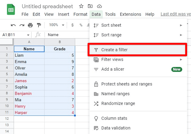
Creating a filter
Step 5: Click on any of these filter icons. A drop-down menu will pop up on your screen. Go to “Sort by color” and select “Text Color” from the side window. Click on any of the two colors to sort the entire set.
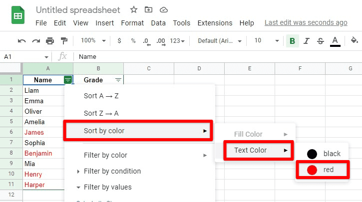
Sorting by text color
If you selected “Red,” red entries would be automatically displayed at the top and vice versa. Also, do not forget that you can repeat the steps mentioned above multiple times for more than two colors.
Sorting cells in Google Sheets by fill color
In the following method, let us assume that you have a specific data set in which particular entries (rows) are filled with a blue color. A classic example would be weather temperature records in different cities. Many weather logging APIs formats these cells with a particular color if they fall below or above some threshold. In this spreadsheet, cities facing negative temperatures have been logged with blue backgrounds. Now, by sorting the cells by fill color, you can immediately group the entire set of cities into two categories.
In the following procedure, we will be displaying ten rows as an example. It might not seem like a good application of sorting these cells by color. However, as the size of your dataset starts to increase, the practicality of this method becomes more evident.
Step 1: Launch your preferred internet browser and go to “Google Sheets.” Log in with your account.
Step 2: From the Google Sheets homepage, open the file in which relevant data is present.
Step 3: Select the entire range of cells with your mouse or a keyboard shortcut. Make sure to include all entries.
Step 4: Click on the “Data” tab from the Google Sheets toolbar. Select “Create a filter” from the drop-down menu. You will notice that the first cell in each column starts displaying a filter icon within it. That indicates filter application.
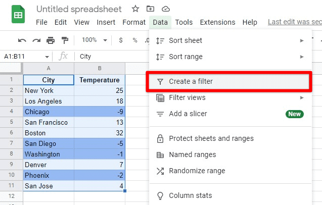
Creating a filter in Google Sheets
Step 5: Click on any of these filter icons. A drop-down menu will pop up on your screen. Go to “Sort by color” and select “Fill Color” from the side window. Next, click on any of the two colors to sort the entire set.
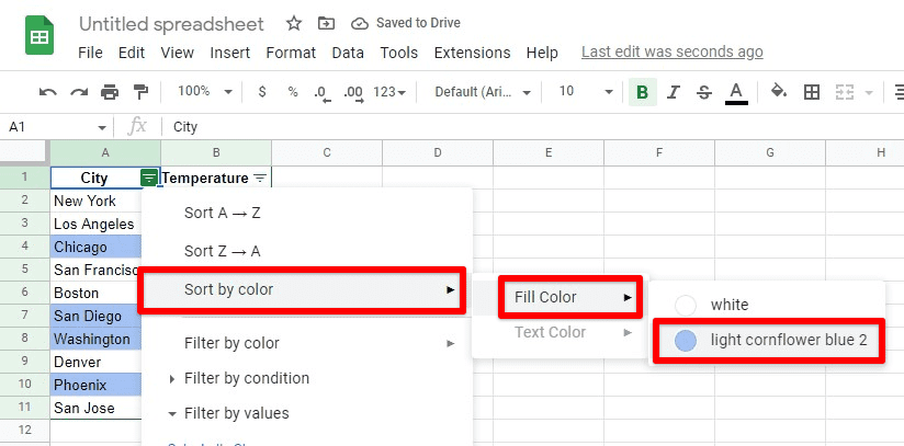
Sorting by fill color
If you selected “Blue,” blue entries would be automatically displayed at the top and vice versa. Also, do not forget that you can repeat the steps mentioned above multiple times for more than two colors.
Unsorting to recover the original sequence
Once you have sorted the data by color, there is a precise approach to unsort it afterward. Without that, you will not be able to recover the original sequence of cells. If you remove the filter, it keeps the data sorted and does not make any changes. The only way you can unsort the data is by creating an additional column of serial numbers for storing the initial order. That has to be done before you apply the filter. When unsorting, select all cells and then choose the column of serial numbers as a sorting reference.
Step 1: Launch your preferred internet browser and go to “Google Sheets.” Log in with your account.
Step 2: From the Google Sheets homepage, open the file in which relevant data is present.
Step 3: Add a new column containing serial numbers with an increment of 1.
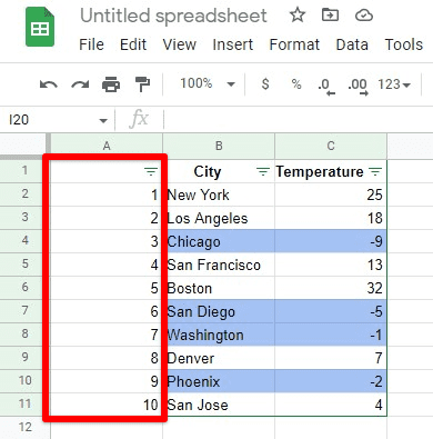
Column of serial numbers
Step 4: Select the entire range of cells with your mouse or a keyboard shortcut. Make sure to include all entries.
Step 5: Sort by color and then sort the entire dataset concerning the column of serial numbers. That would result in a simple unsort, returning your original sequence.
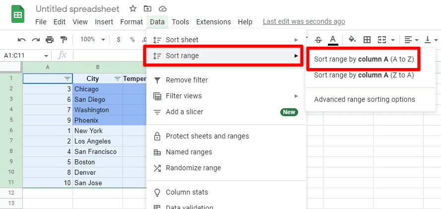
Sorting by a column of serial numbers
Another way to record your initial dataset format is to make a document copy before sorting the rows by color. However, this method is not that practical, especially if you have to deal with multiple arrays at once.
Coloring cells for subsequent sorting
For those with a lot of tabular data, it is not always possible to attain it pre-formatted from the source. If you want to color some cells for subsequent sorting, the most suitable and time-efficient method uses conditional formatting.
This type of formatting usually takes up two distinct forms. One is used for single color while the other generates a color scale. For sorting your data by color, you will be employing the former. It relies on monochromatic formatting in which you change the appearance of a specific cell based on its value. This is for cases when you have a certain threshold for the condition. For example, if you want to sort all cells with numbers greater than 80, you must use single-color conditional formatting.
Step 1: Launch your preferred internet browser and go to “Google Sheets.” Log in with your account.
Step 2: From the Google Sheets homepage, open the file in which relevant data is present.
Step 3: Select the entire range of cells with your mouse or a keyboard shortcut. Make sure to include all entries.
Step 4: Go to the “Format” tab in the Google Sheets toolbar. Click on “Conditional formatting” from the drop-down menu
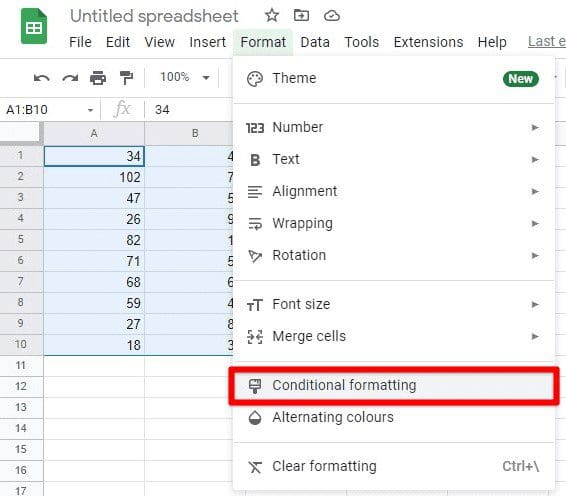
Conditional formatting under the format tab
Step 5: Open the “Conditional format rules” in a new window. Select the “Single color” tab from the top.
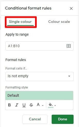
Conditional format rules window
Step 6: Check if the “Apply to range” tab initially contains the cells you selected. If this is not the case, correct the identified range.
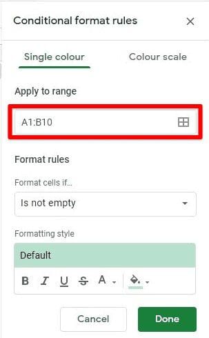
Identifying the correct range
Step 7: Under the “Format cells if” tab, select the “Greater than” option from the drop-down menu—type “80” inside the value bar.
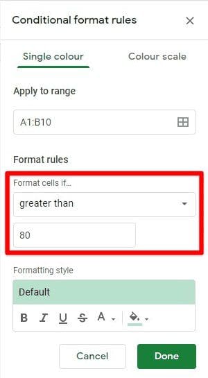
Format cells if value greater than 80
Under the “Formatting style,” you can choose the appearance of filtered cells. After setting up all rules, click the “Done” button to finish the process.
Conclusion
Over the recent years, Google Sheets has transformed itself into a productivity toolbox that can now handle many varied requests and functionalities. Knowing how to sort by color in Google Sheets is a handy trick that proves quite helpful whenever someone wants to organize their data in new, practical ways. Would you like to learn some more functions? Here is a detailed article on finding the average on Google Sheets.
