Google Sheets is an online alternative to MS Excel used to store, edit, and organize tabular forms of data. In such programs, you usually deal with either numbers or strings. When formatting numbers, one might want to find the average of all values stored in a single column. It becomes increasingly difficult to calculate the average manually, especially if there are more than just a few numbers.
In the following article, we will talk about how you can find average on Google Sheets with the help of built-in functions. These functions take up multiple forms and have separate use cases. We will be detailing each one of these variants so that you can decide on which one seems the most suitable and appropriate for specific needs.
Finding the average in Google Sheets
When you have a lot of numbers to work on, the macro implementations can be of great help. To find the average in a single column, you will have to use one of the four corresponding functions. They are named AVERAGE, AVERAGE.WEIGHTED, AVERAGEA, and AVERAGEIF. All four of these functions have separate use cases and slightly differ in syntax.
The AVERAGE function returns the numerical average value in a dataset and ignores any cell that might contain textual contents. More often than not, you will be using this function for simple applications. The remaining three are modeled upon the first to chip in additional functionality. You will find their respective cases and input arguments in subsequent sections. Sheets probably have a lot of features that you do not know about. Read through our guide on how to make QR code in Google Sheets.
Using the AVERAGE function
As described earlier, the AVERAGE function will be your go-to copy in most cases. When you make a call, the input arguments specify the range of cells that contain the numerical data. If the function finds any textual contents within the specified range, it ignores that cell and moves on. Therefore, this function is most suitable if you have different types of data formats within a single sheet or column.
AVERAGE is specified to take a maximum of 30 arguments at once. You can enter these arguments in cellular format or put in the numbers directly. Please note that the AVERAGE function will return the mean of combined arguments. This is because the sum of values in the arguments is divided by the number of cells.
Step 1: Launch your preferred internet browser and go to “Google Sheets.” Log in with your account.
Step 2: Open the file from the Google Sheets homepage in which numerical data is already present.
Step 3: Select a blank cell within the sheet for displaying the calculated average value.
Step 4: Click on the formula bar and type “=AVERAGE(A1:A15)”. Make sure to replace A1 and A15 with the first and last cell numbers in your sheet.
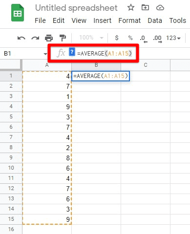
AVERAGE function
Step 5: Press “Enter” or click on any blank space. The cell you selected in Step 3 will start displaying the average of all numbers.
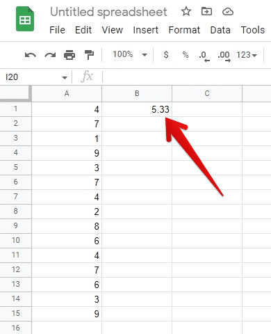
Calculated average
You will notice that the average is represented up to a range of decimal points which are not usually required. To limit the average value to 2 decimal places, select the individual cell and go to Format > Number > Custom Number Format. You can click on the two-point format to apply it immediately.
Using the AVERAGE.WEIGHTED function
Instead of finding a regular average, you might want to calculate the weighted average of your data. However, you will need to provide the corresponding weight and the values—the AVERAGE.WEIGHTED function takes up 2 essential arguments and 2 optional arguments.
The two essential arguments include values and their corresponding weights. Values may refer to a range of cells or contain the values themselves. Similarly, weights may refer to a range of cells or may have the numerical weights themselves. These weights cannot be negative, though they can be zero. Moreover, at least one of the weights in the entire data set must be non-zero. Also, make sure that the range of cells containing the values and their weights have an equal number of entries.
Step 1: Launch your preferred internet browser and go to “Google Sheets.” Log in with your account.
Step 2: Open the file from the Google Sheets homepage in which numerical data (values and weights) is already present.
Step 3: Select a blank cell within the sheet for displaying the calculated weighted average value.
Step 4: Click on the formula bar and type “=AVERAGE.WEIGHTED(A1:A15,B1:B15)”. Ensure to replace A1, A15, B1, and B15 with your sheet’s first and last cell numbers. Column A corresponds to values, whereas column B corresponds to respective weights.

AVERAGE.WEIGHTED function
Step 5: Press “Enter” or click on any blank space. The cell you selected in Step 3 will start displaying the weighted average of all numbers.
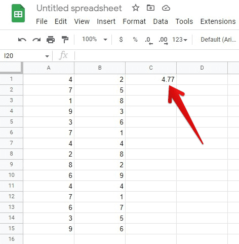
Calculated weighted average
You will notice that the average is represented up to a range of decimal points which are not usually required. To limit the average value to 2 decimal places, select the respective cell and go to Format > Number > Custom Number Format. You can click on the two-point format to apply it immediately.
Using the AVERAGEA function
The AVERAGE function we detailed in the first section skips over the textual data and ignores it completely. However, there is another way to treat these text-based cells within your sheet. The AVERAGEA function considers these specific cells to be containing the number ‘0’. Any text encountered in the value arguments will be 0 and included in the calculation.
AVERAGEA is specified to take a maximum of 30 arguments at once. You can enter these arguments in cellular format or put in the numbers directly. Please note that the AVERAGEA function will return the mean of combined arguments and zero cells. The sum of values in the arguments is divided by the number of cells in the specified range.
Step 1: Launch your preferred internet browser and go to “Google Sheets.” Log in with your account.
Step 2: Open the file from the Google Sheets homepage in which numerical data is already present.
Step 3: Select a blank cell within the sheet for displaying the calculated average value.
Step 4: Click on the formula bar and type “=AVERAGEA(A1:A15)”. Make sure to replace A1 and A15 with the first and last cell numbers in your sheet.
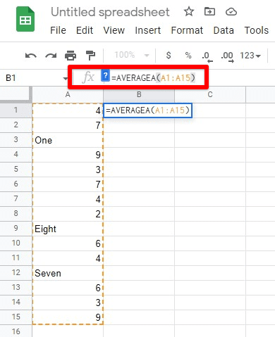
AVERAGEA function
Step 5: Press “Enter” or click on any blank space. The cell you selected in Step 3 will start displaying the average of all numbers.
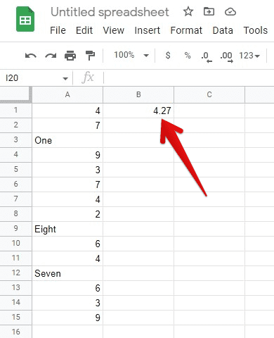
Calculated average with text considered as 0
If your range of cells to be averaged does not contain textual information, then AVERAGE and AVERAGEA functions yield similar results. The AVERAGEA function is used for future-proofing or when numerical inputs are added in strings such as “Nil” or “N/A”.
Using the AVERAGEIF function
Another method for calculating the average in Google Sheets uses the AVERAGEIF function. As evident by its name, this function is used whenever you want to consider cells based on a pre-determined condition or test. Let us say that you need to find the average number of students who passed a certain exam. In that case, you will be putting in a conditional statement that only qualifies those with higher scores than the passing criteria.
The AVERAGEIF function is somewhat different from what you observed previously. It takes in three arguments. These include criteria_range, criterion, and average_range. The critera_range contains the cells which are checked against a specific condition. The criterion is a pattern or test which applies to the cells in criteria_range. Lastly, average_range is a range of cells that is to be averaged. This last argument is optional, and if not included, critera_range is used for the average instead. Here is a detailed article on using conditional formatting in Google Sheets.
Step 1: Launch your preferred internet browser and go to “Google Sheets.” Log in with your account.
Step 2: Open the file from the Google Sheets homepage in which numerical data is already present.
Step 3: Select a blank cell within the sheet for displaying the calculated average value.
Step 4: Click on the formula bar and type “=AVERAGEIF(A1:A15, “>5”)”. Make sure to replace A1 and A15 with the first and last cell numbers in your sheet.
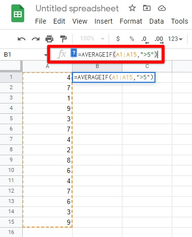
AVERAGEIF function
Step 5: Press “Enter” or click on any blank space. The cell you selected in Step 3 will start displaying the average of all entries greater than 5.
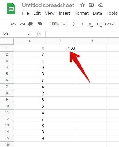
Average of all numbers greater than 5
There are several different criterion categories that the AVERAGEIF function recognizes. Some common conditional statements are listed as follows,
Equal to statement: “text” or number or “=text” or “=number”
Not equal to statement: “<>text” or “<>number”
Greater than statement: “>number”
Greater than or equal to statement: “>=number”
Less than statement: “<number”
Less than or equal to statement: “<=number”
There is another function that resembles in implementation of the AVERAGEIF function. It is called the AVERAGEIFS function. The only thing different in this is that you can use it to check for multiple conditional statements simultaneously. One needs to specify multiple criteria_ranges and multiple tests for each range.
Conclusion
Knowing mathematical functions may save you tons of effort whenever you have to deal with many numerical data within Google Sheets. They perform the same calculations within seconds, which would otherwise take time. One of such functions is the AVERAGE function. It also has three variants employed to find averages in specific circumstances. Are you moving your entire dataset online? Learn how to convert an Excel file to Google Sheets.
