Google Sheets is a powerful software that lets you work on inventive problems and deal with data sets in various ways. One of the possibilities in adding new functionality to your sheet comes with dropdown lists. These lists are handy when collaborating on the same sheet with other team members or colleagues. Whenever an individual uses a sheet for the first time, you would like to ensure the correct approach of operations. That can only be guaranteed with the help of dropdown lists.
Dropdown lists in Google Sheets
Google Sheets is also used to carry forms that can take in information from several users. As you would see on Google Forms or any other information tab, dropdown lists can make sure that only predefined options are selected. Through this approach, you enable yourself to expect certain information in Google Sheets. Moreover, adding dropdown lists to Google Sheets also allows all end-users to fill in the cells rather quickly.
By eliminating the manual input of data, you can save a noticeable amount of effort and time. You can secure a specific list of answers through configured options in these lists. This can be pretty useful in many different applications on Google Sheets, especially if you are integrating it with other platforms.
Surprisingly, creating a dropdown list in Google Sheets is not tricky or complicated. By following a set of simple steps, you can add these lists to your sheet within minutes. With vast usefulness in data entry, dropdown lists are here to stay. By offering the addition of dropdown lists, Google Sheets has enabled its software to remain consistent with the latest capabilities in data management programs.
You can also employ dropdown lists to eliminate any possibility of errors inside Google Sheets. With plenty of functions and formulas used regularly, errors are common. Through dropdown lists, you can safeguard the parameter entries in different functions. Read about using the COUNTIF function in Google Sheets under various applications. Moreover, whenever you need to add in interactive sub-applications inside Google Sheets, dropdown lists can come in as reasonably practical. They can be used in designing collaborative dashboards and charts. These lists can also be employed in changing the contents of a cell for analytic purposes.
Creating a dropdown list of items
Firstly, we will go over the steps you need for creating a dropdown list of items. Once you create one in your sheet, it will give you enough confidence to explore other options with it.
Let us assume that you have created interactive mark sheets for all students enrolled in a particular course. To display the mark sheet of a specific student, you will need a dropdown list with the names of all students. In this tutorial, we will create this list by manually putting in the names. For keeping things simple, we will only consider five names. With a focus on creating this dropdown list, you will have to follow the subsequent steps,
Step 1: Open the desired sheet on “Google Sheets”.
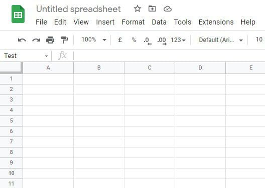
Sheet for the dropdown list of items
Step 2: Select a particular cell where you want to create the dropdown list. Please note that you can also select a range of cells for making multiple lists at once.
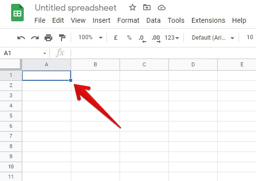
Selecting a cell for a dropdown list of items
Step 3: Click on the “Data” tab from the taskbar. This will open a dropdown menu. Go to “Data validation”.
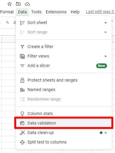
Data validation under data
Step 4: This will pop up the “Data validation” window. Here, you will be able to see many options.
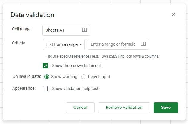
Data validation window
Step 5: From “Criteria”, select “List of items”. Add all names in a comma-separated list in the tab located right in front of criteria options. You can add as many items as you want.
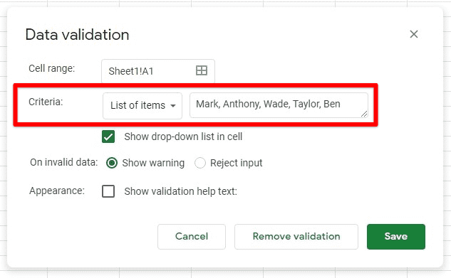
Setting list of items as criteria
Step 6: Make sure that you have ticked the “Show dropdown list in cell” checkbox. If this option is not marked, you will not see the names of students inside the cell.
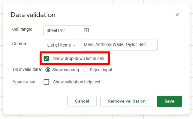
Ticking the dropdown list checkbox
Step 7: From “On invalid data”, select “Show warning”. This will display an error message on the screen every time the user puts in a value, not one of the predefined items. In our case, this will make sure that only those students are added who got enrolled in that course.
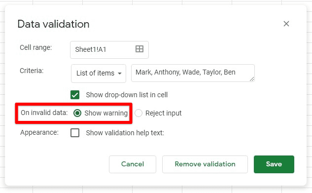
Setting invalid data response
Step 8: Once you have configured the settings for the dropdown list, click on the “Save” button.
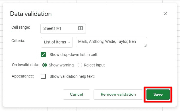
Save button for the dropdown list of items
Now, you can check to see if the list is working as expected. You can launch the dropdown lists and verify the entries one by one. If there are any irregularities, modify the settings by going to “Data validation” again.
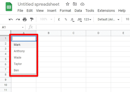
Dropdown list of items
Creating a dropdown list from cells
The other way to create a dropdown list is to take in its items from the contents of the cells in your sheet. This allows you to create dynamic lists that can change their items whenever the information in respective cells changes. This can be particularly useful if you are dealing with shared Google Sheets.
Let us assume that your sheet is filled with vehicle registration numbers collected from a sensor in a parking lot. If you want to create a dynamic dropdown list of these numbers, you will have to make one from a range of cells that contain this information. We will only consider five registration numbers to keep things simple, but that total can scale up to more than a thousand. To create a list for this application, you need to observe the following steps,
Step 1: Open the desired sheet on “Google Sheets”.
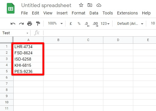
Sheet for dropdown list from cells
Step 2: Select a particular cell where you want to create the dropdown list. Please note that you can also select a range of cells for making multiple lists at once.
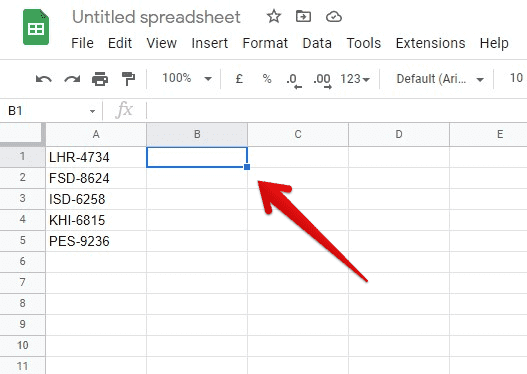
Selecting a cell for dropdown list from cells
Step 3: Click on the “Data” tab from the taskbar. This will open a dropdown menu. Go to “Data validation”.
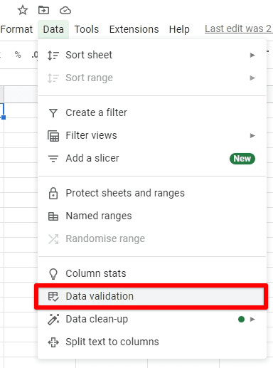
Data validation under data tab
Step 4: This will pop up the “Data validation” window. Here, you will be able to see several options.
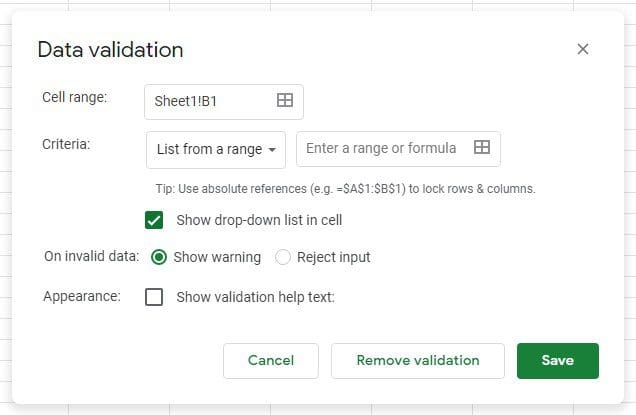
Pop-up data validation window
Step 5: From “Criteria”, select “List from a range”. This will give you a placeholder for adding in the range. You can select the sheet as well as the cells you want. This needs to be defined in a typical range format. You can also click on the table icon and select the cells with your mouse.
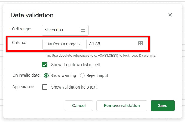
Setting list from a range as criteria
Step 6: Make sure that you have ticked the “Show dropdown list in cell” checkbox. If this option is not marked, you will not see the registration numbers inside the cell.
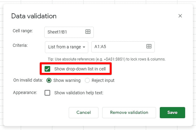
Ticking the show dropdown list checkbox
Step 7: From “On invalid data”, select “Show warning”. This will display an error message on the screen every time the user puts in a value, not one of the predefined items. In our case, this will make sure that only those numbers are added that were detected by the parking sensor.
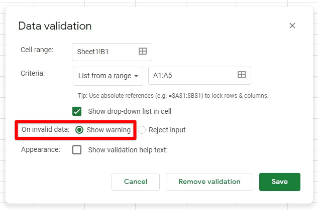
Setting the response to invalid data
Step 8: Once you have configured the settings for this dynamic dropdown list, click on the “Save” button.
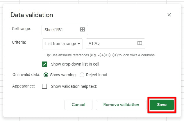
Save button for dropdown list from cells
Now, you can check to see if the list is working as expected. You can launch the dropdown lists and verify the entries one by one. If there are any irregularities, modify the settings by going to “Data validation” again.
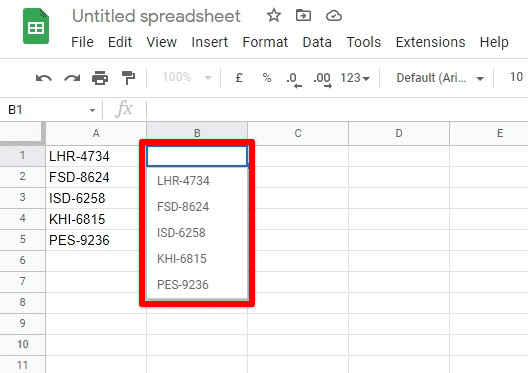
Dropdown list from cells
Formatting a dropdown list
You can also format the cell containing the dropdown list like any other cell in Google Sheets. Formatting the list itself is possible as well. This helps users quickly identify different options from the launched menu. Moreover, you can use conditional formatting for each item on the list. This enables you to link the entries with their cells inside the sheet dynamically. Through conditional formatting, you can color-code your dropdown lists so that they are more visually appealing and functionally effective. For reading all about conditional formatting in Google Sheets, make sure to give this article a read.
For dropdown lists, you can employ formatting through different approaches. The rules are applied only if the text options inside the list match precisely with the one present on any other cell. You can then use different colors to display those cells. Please note that the conditional formatting color scale section can only be explored if all of your dropdown list items are in numerical format. Otherwise, the color scale tab will be automatically disabled for the user.
Conclusion
Adding a dropdown list is the best option whenever you want to put in defined cases in Google Sheets. You can be consistent throughout multiple sheets with no difference whatsoever through them. Moreover, these lists allow your Google Sheets to be more interactive and synergistic. Dropdown lists also enable you to conserve valuable space in Google Sheets. With exquisite data validation, a single cell of your sheet can occupy the contents that would otherwise take hundreds. Moreover, you can benefit from all of this while removing any possibility of incorrect responses. Feel free to go over some more Google Sheets tricks that can prove quite helpful.
