The COUNTIF function in Google Sheets does precisely what its name suggests. It lets you count the number of cells that satisfy a given condition inside the specified range. This incredible functionality enables you to analyze and examine any data set in several different ways. The Google Sheets also comes with an IF condition and a COUNT function. The COUNTIF function is a combination of these two algorithms. It allows you to check a condition on cells while counting their total instances simultaneously.
COUNTIF function in Google Sheets
The COUNTIF function is primarily used in scenarios where you only need to check for one condition. Its syntax is defined to verify a single condition whenever it is implemented. Therefore, you cannot use it whenever more than one condition is checked. In those cases, you need to employ a much similar COUNTIFS function. The COUNTIF function can primarily be divided into two basic functionalities.
One is the conditional statement, whereas the other is the counting algorithm. This function swaps over the specified range and verifies the conditional statement on all cells. If a criterion is met on a cell, the function adds 1 to the count variable. This variable stores the total number of cells that satisfy the given condition. Once the process is completed, the COUNTIF function then displays the result of that count variable inside the cell it was implemented in.
As you now get what COUNTIF does, let us take a brief look at its syntax and how it can be executed in Google Sheets. First, the basic syntax for the COUNTIF function is defined as follows:
=COUNTIF(range, criterion)
In this formula, you can see two parameters for this function. The first is a range, and the second one is a criterion. A range is defined by a group of cells that you need Google Sheets to examine for the criterion. This range can contain cells from a single row, a single column, or multiple rows and columns. There is no upper bound for the range inside a sheet. Theoretically, this means that you can implement COUNTIF on the entire sheet at once. A criterion is any conditional statement that will be checked on all cells. This can deal with numbers, text, references, or expressions. This wide range of statements available for this function allows us to use it in multiple cases.
To deal with cells that contain numbers, you will have to accompany your criterion with greater than (>), less than (<), greater than or equal to (>=), less than or equal to (<=), and not equal to (<>) signs. If you want to work with cell references, you will have to use the ampersand (&) operator before the actual reference. The formula bar in Google Sheets also guides you with fill-in options showing up on your screen as soon as you start typing the formula. This makes the entire process a lot easier for someone using this function for the first time.
When you put in the cell range, Google Sheets will also highlight the included cells in that range. This is done with colored dashed lines that enable you to match ranges with their corresponding entries in the formula bar. If you are working with cells that contain text, you will have to enclose your search criterion in double quotation marks. This lets the program know that you mean to find that string inside cells. If this sounds confusing at first, don’t get worried. You will start getting the hang of it when you see different use cases.
COUNTIF use case with numbers
Most of the time, Google Sheets is filled with data that is in numerical format. Therefore, you need to know how to use COUNTIF with numbers. Let us assume that you have a set of cells that contain numbers in both negative and positive ranges. You need to find out the number of cells with a negative number inside them. For this, you will have to take the following steps,
Step 1: Open the desired sheet on “Google Sheets.”
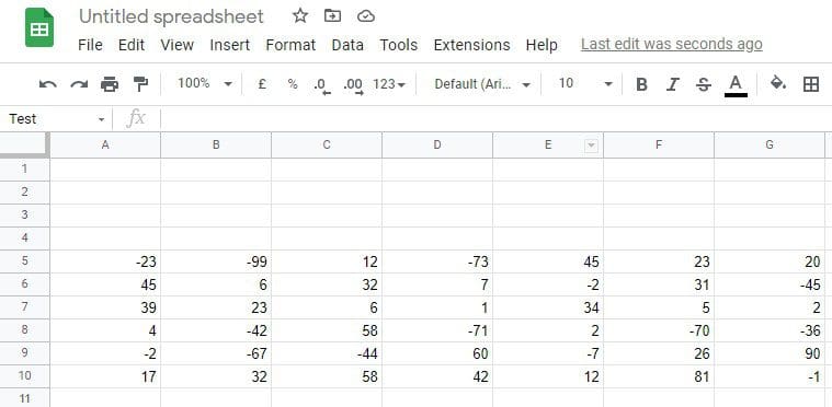
Google Sheets for the numerical use case
Step 2: Select that particular cell inside the sheet where you want to display the result. The result, in this case, will be the total number of cells with negative integers.
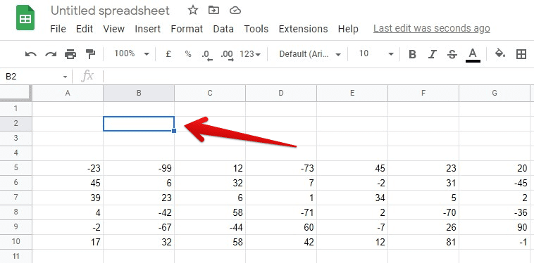
Selecting a cell for the numerical use case
Step 3: Type “=COUNTIF(A5:G10,”<0”)” in the “Formula Bar.” Press the Enter key. Make sure to replace A5:G10 with the range of cells you are interested in.
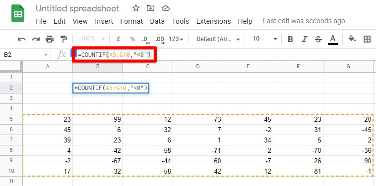
Implementing COUNTIF function for the numerical use case
Step 4: After you press the Enter key, the cell you selected will display the number of cells with negative integers.
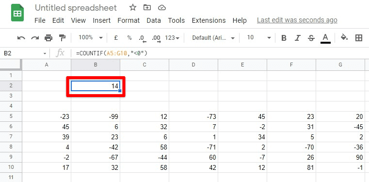
Number of cells with negative integers
You can use the same procedure to employ all sorts of conditions on numbers. This allows you to maximize the functionality in so many ways. For example, you need to know that you do not have to type quotation marks when looking for an exact number. In that case, all you require to do is type in that particular number as the second parameter of the COUNTIF function.
COUNTIF use case with text
Many a time, the data in Google Sheets is in textual format. What’s great about the COUNTIF function is that it also works perfectly well with text-filled cells. Using this function, you can count the total number of times a string is repeated in a range of cells. You can also use the same method to find out the number of cells with an empty string. This is one of the methods we use in counting the number of blank cells in Google Sheets. Let us assume that you have the favorite NFL teams of all students enrolled in a particular class. You need to find out the number of students like the Kansas City Chiefs. For this, the following steps will have to be observed,
Step 1: Open the desired sheet on “Google Sheets.”
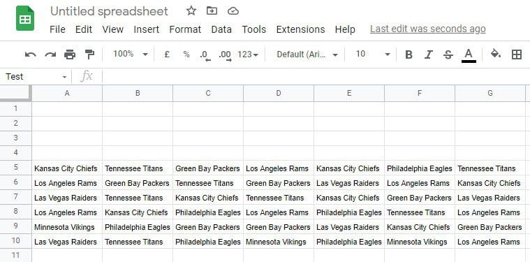
Google Sheets for the textual use case
Step 2: Select that particular cell inside the sheet where you want to display the result. The result, in this case, will be the total number of cells with Kansas City Chiefs written inside them.
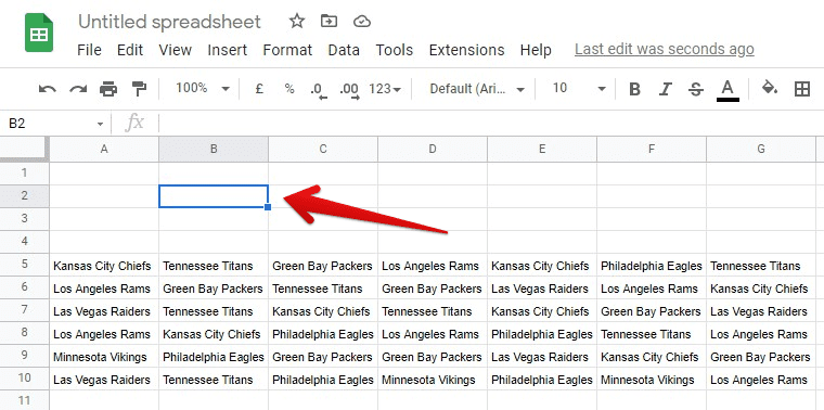
Selecting a cell for the textual use case
Step 3: Type “=COUNTIF(A5:G10,”Kansas City Chiefs”)” in the “Formula Bar.” Press the Enter key. Make sure to replace A5:G10 with the range of cells you are interested in.
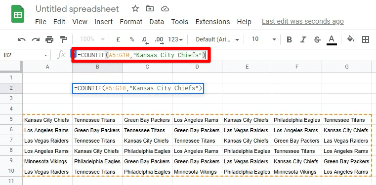
Implementing COUNTIF function for the textual use case
Step 4: After you press the Enter key, the cell you selected will display the number of students like Kansas City Chiefs.
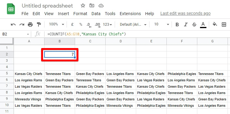
Number of students who like Kansas City Chiefs
The same procedure can be applied to determine the total number of instances for any string, even a blank one. Remember that whether you are dealing with numbers, text strings, or references, the value that the COUNTIF function returns will always be numerical. This allows you to use the COUNTIF function in other mathematical expressions. Moreover, you can also use this function multiple times in a single formula.
COUNTIF use case with references
A reference to a cell can be considered as its address. We can only differentiate one reference from the other using these addresses. If a cell is identified with the B7 identifier, then we can use its reference to access the content placed inside that cell. For example, if the cell B7 contains 42, then typing &B7 in a formula would mean the same thing as 42. The keyword (&) dereferences the identifier and is considered a pointer to the cell where this information is present. This is a beneficial use case of the COUNTIF function. Let us assume that you want to see how many students scored higher than a particular student in a class. It would help if you referenced the marks of that student and then compared it with everyone else. For this, the following steps are required,
Step 1: Open the desired sheet on “Google Sheets.”
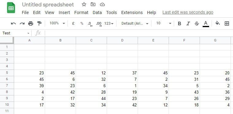
Google Sheets for the reference use case
Step 2: Select that particular cell inside the sheet where you want to display the result. The result, in this case, will be the total number of students who scored higher than, let’s say, Michael.
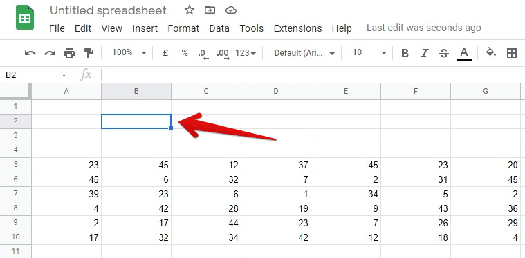
Selecting a cell for the reference use case
Step 3: Type “=COUNTIF(A5:G10, “>” & B7)” in the “Formula Bar.” Press the Enter key. Make sure to replace A5:G10 with the range of cells you are interested in.
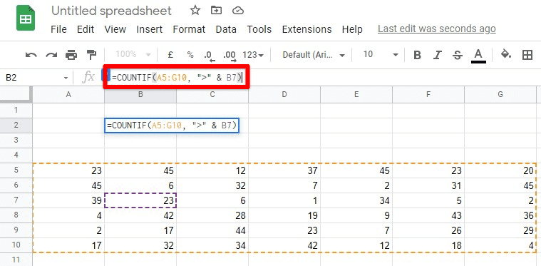
Implementing COUNTIF function for the reference use case
Step 4: After you press the Enter key, the cell you selected will display the number of students who scored higher than Michael.
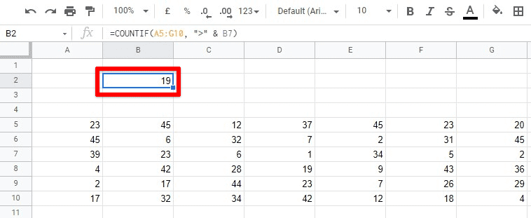
Number of students who scored higher than Michael
With referencing, you can make your function calls to be more dynamic. Even if the entry in the cell changes over time, the function would still work perfectly well with the new values.
Conclusion
With conditions that work with multiple data formats, the COUNTIF function has optimized data analytics in Google Sheets. Knowing how to use the COUNTIF function in Google Sheets lets you handle varying scenarios. With the syntax and concept learned, you can move on to develop ingenious yet simple solutions for the data in your sheets. This enables you to find time-saving and practical approaches to handling data that would have been impossible otherwise. It makes your experience with this software a lot more efficient and capable. Here are 10 helpful Google Sheets tricks for you if you are interested.
