If you are working with data in Google Sheets, you will have a great tool under your belt in the form of conditional formatting. With this technique, you can format multiple cells in Google Sheets without editing them manually. Follow this link to find other helpful Google Sheets tricks. Conditional formatting allows you to highlight different aspects in your sheet within moments.
The idea behind conditional formatting is to use the data stored in cells as a condition for their customization. This means that you can display distinct categories of cells differently. Conditional formatting proves to be quite helpful in data analytics and examination. This can do wonders for minimizing the time you spend on formatting Google Sheets cells.
Conditional formatting in Google Sheets
The technique of conditional formatting was developed for Excel sheets originally. This formatting method enables users to achieve higher functionality with minimal effort. Before we dive into different use cases, let us look at where this tool is located and how it can be accessed. You will find the conditional formatting tool under the “Format” tab in the taskbar. As you click on the “Conditional formatting” tab, a panel will be opened on the right side of your screen. This panel contains all rules and conditions that can be adjusted for a particular sheet. In this panel, you can see two main tabs. One is for single color options, while the other reads color scale.
As the name suggests, a single color tab is for monochromatic formatting in which you format a specific cell based on its value. This is for cases when you have a certain threshold for the condition. For example, if you want to color all cells containing a number under 50, you will have to go for single color conditional formatting. With this, a cell containing 49 and a cell containing 1 will be colored similarly. On the other hand, a color scale divides your condition into multiple categories.
You can represent different number ranges with varying shades of the same color through color scaling. This can transform your sheet into a color-coded map that is visually appealing and conveys the general trend in a single sight. In this case, you can set the cells to be formatted with increasingly bright and sharp colors as their value rises. Conditional formatting can also be used to highlight blank cells in a sheet. Read this article on how to count blank cells on Google Sheets. For the sake of this tutorial, we are going to go over three use cases for conditional formatting in Google Sheets. Let us take a brief look at each one of these applications one by one.
Highlighting cells above a specific value
In this use case, we will assume that you have the data from a car speedometer during the entire length of a day. We need to figure out the number of times the car went above the speeding limit. In our example, you will only see values in 20 cells. But if this is perceived as a real-world problem, then the actual values can take hundreds of thousands of cells.
Under those circumstances, it would not be possible for anyone to find overspeeding instances manually. Therefore, your only option would be to use conditional formatting. To highlight all cells containing speedometer values above 80, you will have to observe the following steps,
Step 1: Open the desired sheet on “Google Sheets”.

Sheet with speedometer values
Step 2: Use your mouse to select all cells that comprise your data set.

Selecting all speedometer values
Step 3: Go to the “Format” tab in the taskbar. From the drop-down menu, click on “Conditional formatting”.
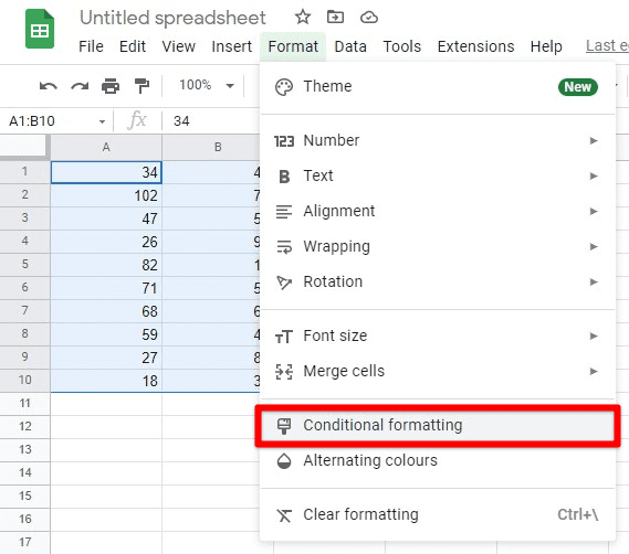
Conditional formatting under format
Step 4: This will open up the “Conditional format rules” in a new window. Select the “Single color” tab from the top.
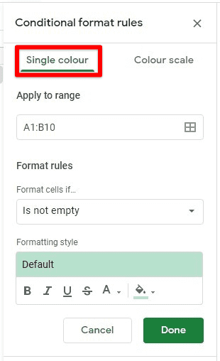
Conditional format rules
Step 5: Check if the “Apply to range” tab contains the cells you selected in the beginning. If this is not the case, make sure to correct the identified range.
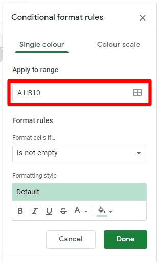
Identifying correct range
Step 6: Under the “Format cells if” tab, select the “Greater than” option from the drop-down menu—type “80” inside the value bar.
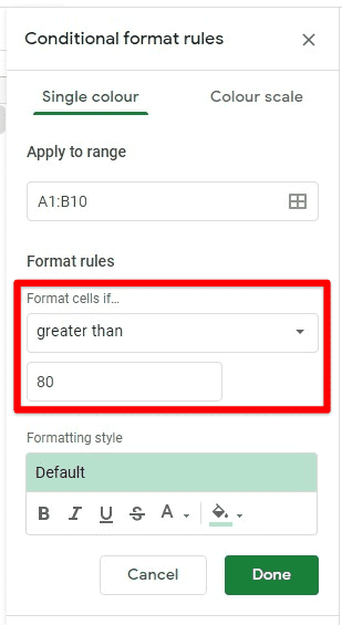
Format cells if value greater than 80
Step 7: Under the “Formatting style”, you can choose the appearance of cells that contain values above 80. Since we are dealing with speeding, let us select the red color.
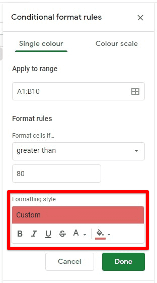
Coloring the cells red
Step 8: After setting up all rules, you can click on the “Done” button. All cells with values above 80 will be colored red immediately.
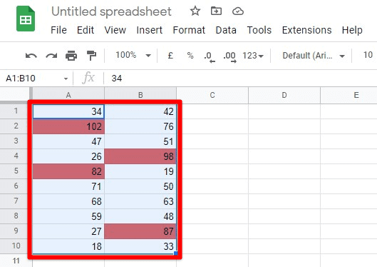
Conditionally formatted speedometer values
Coloring cells for a range of values
In this use case, we will assume that you have the data from a temperature sensor installed inside a boiler at a factory. You do not need to color cells containing a number above or below a particular threshold for this application. Instead, we are looking for a heatmap that allows you to visualize the overall temperature trends. Since we are dealing with temperature values, we would like to represent lower values with green and higher values with red. Once formatted, you can use this sheet to observe temperature values during different times throughout the day.
In our example, you will only see values in 20 cells. But if this is perceived as a real-world problem, then the actual values can take hundreds of thousands of cells. Under those circumstances, it would not be possible for anyone to observe mass trends without color-coding the cells. Therefore, your only option would be to use conditional formatting. To color cells concerning their values, you will have to follow the subsequent steps,
Step 1: Open the desired sheet on “Google Sheets”.
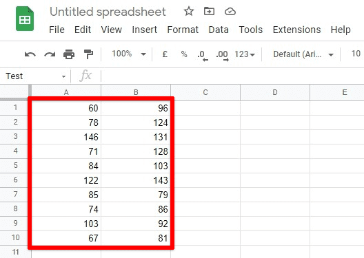
Sheet with temperature sensor values
Step 2: Use your mouse to select all cells that comprise your data set.
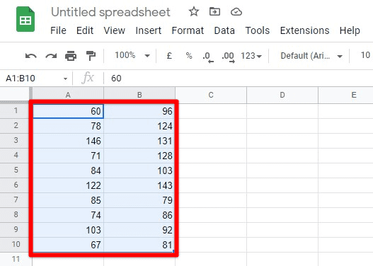
Selecting all temperature sensor values
Step 3: Go to the “Format” tab in the taskbar. From the drop-down menu, click on “Conditional formatting”.
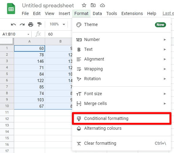
Conditional formatting under the format tab
Step 4: This will open up the “Conditional format rules” in a new window. Select the “Color scale” tab from the top.
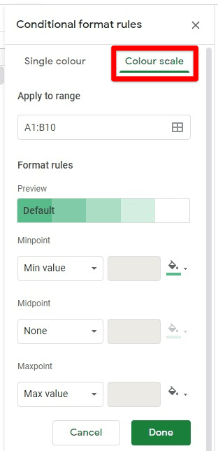
Conditional format rules and color scale
Step 5: Check if the “Apply to range” tab contains the cells you selected in the beginning. If this is not the case, make sure to correct the identified range.
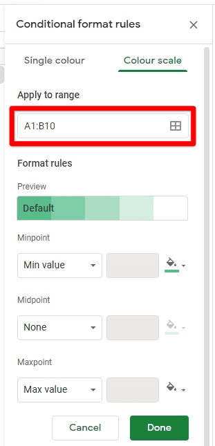
Selecting the correct range
Step 6: Under the “Preview” tab, select any color palette that you would like for your sheet. In these palettes, the colors present on the left side are applied to lower value cells, and colors present on the right side are used to higher value cells.
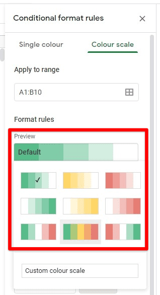
Selecting color palette
Note: You can also make your own color choices if you want. The format rules provide you with the option to select three colors for minimum, central, and maximum values. All other colors between these values are extrapolated with a fine gradient. The percentile for the middle value can also be adjusted.
Step 7: After setting up all rules, you can click on the “Done” button. The cells you selected, in the beginning, will now be colored concerning their values.
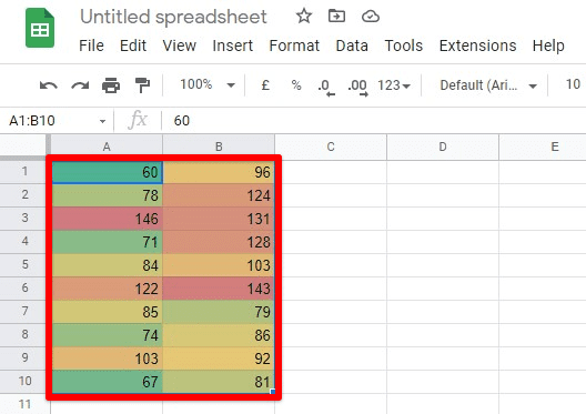
Color-coded temperature sensor values
Finding cells with a search item
In this use case, we will assume that you have the names of all students enrolled in a specific course. If you want to search for a particular student, you can enter their name inside the sheet, and the name will automatically highlight itself. This functionality can only be added with the help of conditional formatting. As you would have already imagined, this will only highlight those instances that match the searched item.
In our example, you will only see names in 10 cells. But if this is perceived as a real-world problem, then the actual names can occupy hundreds of cells. Under those circumstances, it would be tough for us to find a student manually. Therefore, the only option is to use conditional formatting. To highlight cells that match with the searched name, you will have to follow the steps explained below,
Step 1: Open the desired sheet on “Google Sheets”.
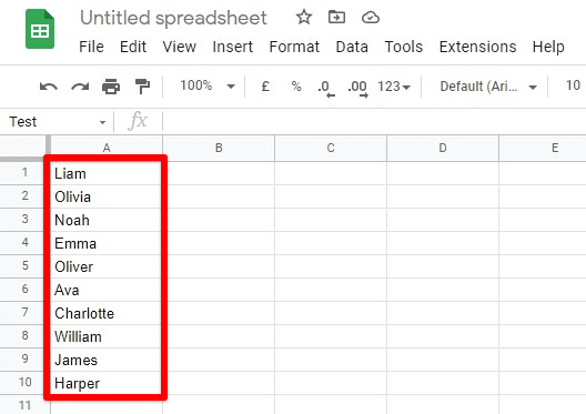
Sheet with student names
Step 2: Use your mouse to select all cells that comprise your data set.
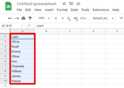
Selecting all names
Step 3: Go to the “Format” tab in the taskbar. From the drop-down menu, click on “Conditional formatting”.
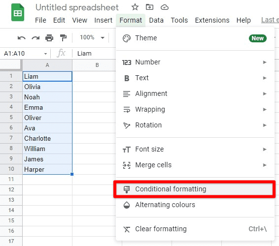
Opening conditional formatting from the taskbar
Step 4: This will open up the “Conditional format rules” in a new window. Select the “Single color” tab from the top.
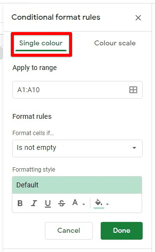
Conditional format rules and single color
Step 5: Check if the “Apply to range” tab contains the cells you selected in the beginning. If this is not the case, make sure to correct the identified range.
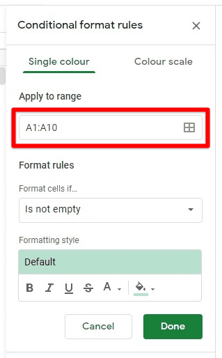
Ensuring correct range
Step 6: Under the “Format cells if” tab, select the “Custom formula” option from the drop-down menu.
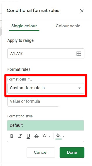
Setting the condition type.
Step 7: Type “=AND(NOT(ISBLANK($C$1)),ISNUMBER(SEARCH($C$1,A1)))” inside the formula bar. Kindly note that the cell used for searching is C1. You can change it if you want.
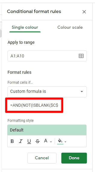
Implementing the custom formula
Step 8: Under the “Formatting style”, you can choose the appearance of cells to be highlighted. Let us pick the green color.
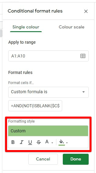
Formatting the searched cell
Step 9: After setting up all rules, you can click on the “Done” button. Now, whenever you type a name in cell C1, the respective cell containing that name will be automatically highlighted.
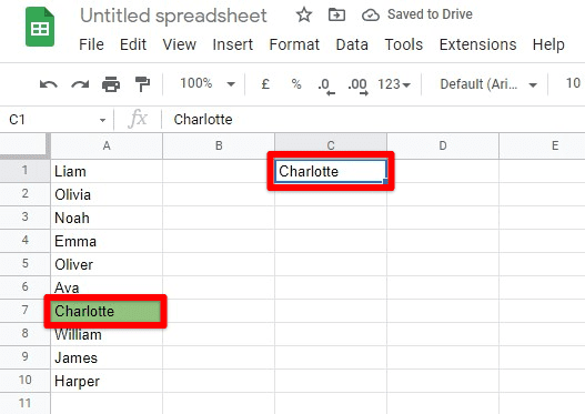
Searching for Charlotte
Conclusion
You can use conditional formatting to organize the data present in Google Sheets. It is beneficial for data analytics and visuals. The customization offered by this feature is truly unique, which shows you the real power Google Sheets brings into your working routine. Moreover, this type of data formatting can also support other functions in the Google Sheets library. In this article, you can read all about using the COUNTIF function.
